| Issue |
Ann. Limnol. - Int. J. Lim.
Volume 56, 2020
|
|
|---|---|---|
| Article Number | 13 | |
| Number of page(s) | 12 | |
| DOI | https://doi.org/10.1051/limn/2020010 | |
| Published online | 04 June 2020 | |
Research Article
Effect of sample size on habitat suitability estimation using random forests: a case of bluegill, Lepomis macrochirus
Department of Civil and Environmental Engineering, School of Environment and Society, Tokyo Institute of Technology, 2-12-1-M1-4, Ookayama, Meguro-ku, Tokyo 152-8552, Japan
* Corresponding author: This email address is being protected from spambots. You need JavaScript enabled to view it.
Received:
17
December
2019
Accepted:
13
April
2020
Abstract
Species distribution models (SDMs) have been used to understand the habitat suitability of key species. Habitat suitability plots, one outcome from SDMs, are valuable for understanding the habitat suitability and behavior of organisms. The sample size is often constrained by budget and time, and could largely influence the reliability of habitat suitability plots. To understand the effect of sample size on habitat suitability plots, the present study utilized random forests (RF) combined with partial dependence function. And the bluegill (Lepomis macrochirus), a main exotic fish species in the Japan rivers, was selected as target species in this study. Total of 1010 samples of bluegill observations along with four environmental variables were surveyed by the National Censuses on River Environments. The area under curves was calculated after generating RF models, to assess the predictive model performance, and this process was repeated 1000 times. To draw habitat suitability plots, we applied partial dependence function to the formulated RF models, and 15 different sample sizes were set to examine the effect on habitat suitability plots. We concluded that habitat suitability plots are affected by sample size and prediction performance. Notably, habitat suitability plots drawn from the sample size of 50 greatly varied among the 1000-time iterations, and they are all different from the observations. Furthermore, to deal with the case of limited samples, we proposed a novel approach “averaged habitat suitability plot” for delineating habitat suitability plots. The proposed approach enables us to assess the habitat suitability even with a small sample size.
Key words: Species distribution model / partial dependence function / Bluegill / habitat suitability / random forests
© EDP Sciences, 2020
1 Introduction
Species distribution models (SDMs) are important tools for describing the relation of species observation with environmental variables (Guisan and Thuiller, 2005). In former studies, SDMs were used for various purposes such as quantifying biodiversity distribution and assessing climate change effect on species distribution (Cheung et al., 2009; Hermoso et al., 2015; Rydgren et al., 2003; Ryo et al., 2018). The increasing availability of environmental databases and the recent improvement of computational technologies (Barbosa and Schneck, 2015) enable us to apply machine learning approaches (e.g., random forests (RF; Breiman 2001) and generalized boosted regression models (GBM; Friedman et al., 2000) for ecological study and environmental management (Conti et al., 2015; Hopkins and Roush, 2013). As a result, the last decade has seen a surge in the development of SDMs (Guisan et al., 2013b). Compared to conventional SDMs, such as generalized linear model (GLM; Nelder and Wedderburn, 1972) and generalized additive models (GAM; Hastie, 2017), machine learning approaches (e.g., RF and GBM) do not require assumptions regarding population distributions and estimate parameters directly from empirical data (Shiroyama and Yoshimura, 2016). However, the complexity of machine learning approaches complicates the interpretation of the relationship between response variables with environmental variables, as this relationship is put into a “black-box” (Elith et al., 2008).
The visualization of species' responses to environmental variables is valuable for understanding habitat suitability and behavior of organisms (Mi et al., 2017b; Michaelis and Diekmann, 2017; Muñoz-mas et al., 2016; Olden et al., 2004; Vezza et al., 2015; Zurell et al., 2012). These generated plots were referred to as ‘prediction curves,’ ‘response curves,’ ‘species response curves,’ and ‘habitat preference curves’ in previous studies (Austin, 2002; Fukuda, 2011; Rydgren et al., 2003). For simplicity, we collectively refer to these terms as ‘habitat suitability plot.’ Machine learning or statistical algorithms are used to formulate prediction models and are combined with visualization techniques (e.g., partial dependence function, averaging methods) to draw habitat suitability plots. Shiroyama and Yoshimura (2016) have assessed the applicability of partial dependence function combined with five different modelling algorithms. The result illustrated that the combination of partial dependence function and RF reasonably describe the habitat suitability of the bluegill, Lepomis macrochirus Rafinesque.
The accuracy of SDMs relies on sample size (Guisan et al., 2013a). There are many reasons why model performance is generally affected by sample size. For example, the level of uncertainty associated with parameter estimation decreases with increasing sample sizes. When sample sizes are small, outliers carry more weight in analytics (Wisz et al., 2008). In practice, the number of samples used in modelling varies from ten to thousands of cases. Thus, it is important to investigate how sample size affects model predictive performance (Kim, 2009; Moudrý and Šímová, 2012). Recent studies have investigated the relationship between sample size and prediction accuracy of the SDMs. The application of 12 modelling algorithms to three sample sizes (100, 30 and 10 observations) encouraged conservative use of prediction models generated using small sample size (Wisz et al., 2008). Stockwell and Peterson (2002) insisted that machine learning algorithms showed nearly the same accuracy for cases of 100 and 50 observations. Moreover, the comparison of the prediction models with sample sizes ranging from 30 to 2500 observations concluded that models with a sample size of 200 and lower tend to yield inaccurate predictions (Hanberry et al., 2012). Despite the fact that the sample size affects the predictive performance of the models, many researchers have generated habitat suitability plots without addressing this issue. The relationship between habitat suitability plots and the sample size is critically important because the number of samples available for generating predictions is often constrained by available budget and time (Hanberry et al., 2012; Moudrý and Šímová, 2012; Wisz et al., 2008).
Given the background, the present study aimed to investigate the effect of sample size on habitat suitability plots using random forests. The target species was the bluegill, Lepomis macrochirus, which is an exotic fish species in rivers in Japan. To achieve this objective, we focused on (1) understanding the effect of sample size on the predictive model performance, (2) examining the effect of sample size on habitat suitability plots, and (3) proposing a practical method for delineating habitat suitability plots in case sample size is limited. In this study, we applied a combination of RF and partial dependence function to draw habitat suitability plots.
2 Study region and dataset
2.1 Study region and monitored data
In this study, seven rivers in the Kanto region (Onishi, 2013), Japan, were selected for model construction and habitat suitability assessment of the bluegill (Fig. S1, Tab. S1). This region has a large plane in the central part and mountain area in northwest. All the data used in this study were collected from National Censuses on River Environments (NCRE) of Japan. This survey has been conducted by the Ministry of Land, Infrastructure, Transport and Tourism (MLIT) of Japan since 1990 (MLIT, 2011), and aims to monitor riverine species distribution and apply the collected data to river management and to promote ecological research on the riverine ecosystem (MLIT, 2006). NCRE records the presence and absence of the riverine species (e.g., fish, invertebrates, birds, plants, etc.) and relevant environmental variables of 109 Class-A rivers once in every five years (fish and invertebrates) or every ten years (the other riverine species). This survey is conducted from spring to autumn at least two times in each river. The timing and frequency of the survey are determined based on the ecology of target community and climate condition (MLIT, 2006). In each river, environmental variables and presence/absence of the riverine species were monitored at each sampling spot (MLIT, 2006b). In the present study, the number of observations collected from 2006 to 2010 was 1010. Throughout the analyses, we included four environmental variables: longitudinal slope, water depth, velocity, and water temperature at each of the sampling spots (Fig. S2, Tab. S2). There are three interactive resistance mechanisms in the invasion process by exotic species: environmental resistance such as temperature and flow, biotic resistance and demographic resistance, and environmental resistance is considered as the most critical in determine the outcome of the invasions (Moyle and Light, 1996). Therefore, only environmental variables were incorporated in this research.
2.2 Target fish
This study targeted the bluegill, Lepomis macrochirus, which is native to the Lake Champlain and southern Ontario regions (Stuber et al., 1982), and is exotic in Japan. The bluegill was introduced in Japan in the 19th century for recreational purposes, such as fishing, and are now colonized across Japan. Its spawning period spans from June to August in Japan (Nakao et al., 2005). The bluegill is an omnivorous fish; they feed on waterweed and algae, and prey on various aquatic fauna such as invertebrates, fish eggs, and juveniles of other fish (Kawanabe et al., 2013). Bluegills' dominance, in particular their predation pressure on zooplankton, is one of the causes for declining native fish in lakes (Taniguchi, 2012).
In NCRE, the bluegill was captured by using cast net and hand net. Additionally, other tools, such as drift nets, gill nets and electrofishing, were applied depending on the hydraulic condition of the investigative spots (MLIT, 2006a). The bluegill were observed at 25% of the observations in the Tone River, followed by the Kuji River (19%) and the Naka River (10%). In total, the bluegill was observed at 15% of all the observed spots (Tab. S1).
3 Methods
3.1 Random forests
Random forests (RF) (Breiman, 2001) was used to model the relationship between bluegills' presence/absence and environmental variables. RF is a supervised machine learning method based on decision tree, taking the average of a large number of trees (thus called “forest”) which are built through randomly finding and splitting feature nodes (hence called “random”). It is capable of dealing with nonlinear relationships where data with complex interactions. This model is a popular algorithm due to its easy applicability to classification and regression problems (Hapfelmeier and Ulm, 2013). RF generates a large number of trees using different bootstrapped samples, and then combines the predictions from all the trees to produce accurate predictions (Cutler et al., 2007; Hanberry et al., 2012). The predictions derived from this algorithm are stable even if the dataset have both outliers and noise, and have a potential to show high prediction accuracy compared to conventional statistical approaches (Breiman, 2001; Cutler et al., 2007; Mi et al., 2017a).
This high performance is generated by reducing the correlation among generated trees. This is achieved by randomly selecting the input variables; before growing a tree using a bootstrapped dataset, select m (m ≤ p) variables at random from all the variables, where p is a total number of variables in an original dataset (Hastie et al., 2009). All analyses were implemented in R software (R Development Core Team, 2014, version 3.1.1). The randomForest package (Liaw and Wiener, 2015) was used for RF formulation.
In the random Forest package, m is set as  at classification and p/3 for regression in default (Liaw and Wiener, 2015). In this research, the value of m was selected using the grid searching algorithms using the caret package (Kuhn et al., 2016). In addition, we generated 500 trees, which is the default in randomForest package, for each RF model.
3.2 Habitat suitability plots (partial dependence function)
Machine learning algorithms are more common, especially when dealing with large observational datasets. However, these algorithms do not produce simple prediction formulas such as linear regressions. Thus, it can be challenging to understand the results and explain processes modelled (Greenwell, 2017). Partial dependence function (Friedman, 2001) can serve as a low dimensional graphical rendering to reveal the relationship between the response and a subset of predictors (typically 1–3) of interest. In linear regression models, the coefficients are estimated to indicate the average effect on Y of a one-unit increase of Xj while holding all other predictors fixed. The interpretation by partial dependence function works in a similar manner. The partial dependence function fS(XS) is defined as follows (Hastie et al., 2009): (1)
(1)
where X T = (X1, X2,…, Xp) is a matrix (p × n) of input variables (p, the number of environmental variables; n, total number of samples). Xp = {Xp,1, Xp,2, … , Xp,n} is the subvector of the input variables. f(X) describes the dependence of X, as calculated by random forests, and E [f (X)] is the expected value of f(X). XS is the subvector of the input variable with S ⊂ {1, 2,…, p}. C is a complement set such that S ∪ C = {1, 2, … , p }.
In practice, Let the complete dataset of predictors in the model be X = {X1, X2,… , Xp} and the dataset of response variable be Y. For simplification, let X be the predictor of interest with values {X1,1, X1,2,… , X1,n}, (e.g. X1 = {X1,1 = 1, X1,2 = 3, X1,3 = 4, X1,4 = 3, X1,5 = 10, X1,6 = 1} (n = 6), and all unique values in X1 are in the vector x1 = {X1,1, X1,2,… , X1,k} (k is the number of distinct values in X1) (e.g. x1={x1,1 = 1, x1,2 = 3, x1,3 = 4, x1,4 = 5, x1,5 = 10} (k = 5)). The partial dependence of Y on X1 is constructed using the following algorithm:
- 1.
For i ∈ {1, 2,… , k},
- i.
Replace the original values of X1 with the constant x 1,i in dataset X, keeping the original values of other predictors;
- ii.
Compute predicted values using the modified dataset and generate the vector of those predicted values;
- iii.
Calculate the average prediction, denoted by y1,i.
- i.
- 2.
Plot the pairs {x1,i, y1,i} for i = 1, 2,… , k.
The above procedure can be applied to each predictors of interest. In this study, partial dependence function was used to draw habitat suitability plots combined with the formulated RF models. Within the algorithm described above, n and p were set at 1010 and 4, respectively, and S was set at one for partial dependence on individual variables. Throughout the analyses, we referred the results of plots drawn by partial dependence function as habitat suitability plot.
3.3 The effect of sample size on accuracy of habitat suitability
3.3.1 Sample size effect on model performance
The observation data (n = 1010) were randomly divided into two groups: training data (n = 900) and test data (n = 110) (Fig. 1A). To compare the prediction performance of various sample sizes, 14 different sample sizes were generated; sample sizes from 900 to 100 (i.e., 900, 800, 700, 600, 500, 400, 300, 200, and 100). Similarly, sample sizes from 100 to 50 (i.e., 90, 80, 70, 60, and 50) were also generated. Each subset of the observation data was randomly selected without replacement.
As the next step, these 14 datasets were individually used to formulate RF model. Then, for each generated models, we calculated the area under the receiver operating characteristic curve (AUC) as a performance measure (Fielding and Bell, 1992). Receiver Operating Characteristics (ROC) is a way of visualizing the performance of a binary classifier, which has an increasing use in machine learning recent years ( Fawcett, 2006). Considering a classifier that generates only two classes: positive or negative, the true positive rate (TPR, also called recall and sensitivity) is the percentage of positive instances that are correctly identified as positive, while the false positive rate (FPR) is the proportion of negative instances that are wrongly identified as positive. The FPR equals to one minus the true negative rate (also called specificity). ROC graph is a two-dimensional graph where the true positive rate is Y axis and the false positive rate is on X axis. The closer the curve is to the northwest, the better the classifier preforms. To make a comparison among different models, a common method is to calculate the area under the ROC curve, simplified as AUC. Since the area of the ROC space is 1, the value of AUC is between 0 and 1. AUC indicates the predictive ability for presence/absence of a species. For instance, an AUC of more than 0.9 indicates that the presence and absence are accurately discriminated. While an AUC of 0.7–0.9 indicates moderately useful models, the range less than 0.7 indicates that the model does not have the ability to discriminate (Swets, 1988). Test data (n = 110) were not used for modelling; thus, the high AUC of test data indicates high predictive accuracy for unseen data. We iterated all of these processes 1000 times, and calculated means and standard deviations of AUC for each sample size.
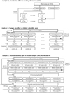 |
Fig. 1 Flowchart describing the analyses of this study. PCC indicate Pearson's correlation coefficient. |
3.3.2 Sample size effect on habitat suitability plots
3.3.2.1 Mean Pearson's correlation coefficient with 1000 iterations
The sample size effect on habitat suitability plot was investigated using following steps. Similar to Analysis A, the datasets of 14 different sample sizes were generated from all the observations (n = 1010) by random selection without replacement. Then, these 14 sample sizes as well as full samples model (n = 1010) were individually fitted using RF algorithms with parameter fitting (Fig. 1B).
Next, habitat suitability plots were generated by combining formulated RF models with partial dependence function. For each sample size, habitat suitability plots were delineated for each of four environmental variables (i.e., depth, temperature, slope, and velocity). They were compared to the observed ratio of the presence in order to determine whether the estimated habitat suitability plots accurately described the observed bluegill distribution. The estimated habitat suitability plots and the observed ratio of presence were standardized, and Pearson's correlation coefficient (PCC) and its p-value were calculated as performance measures. All of these processes were iterated 1000 times, and the mean PCC of those iterations was calculated for each sample size.
3.3.2.2 Averaged habitat suitability plot
Here, we present a novel method to draw habitat suitability plot from limited data, which is named averaged habitat suitability plot. First, an observed range of a target variable was divided into several points. For example, if the observed range of water depth is from 0 to 100 cm, then this range is divided into three points, such as 0, 50, and 100 cm. Next, several habitat suitability plots are generated through iteration process; in Analysis B-2, 1000 habitat suitability plot were made (Fig. 1B). This indicates that after drawing multiple habitat suitability plots, there are multiple estimated values for each point of the variable. Finally, the estimated values of each point are averaged and then these averaged values are connected, which is averaged habitat suitability plot.
In Analysis B-2, PCC between each averaged habitat suitability plot and the observed ratio of presence were also calculated. Finally, PCC of the averaged habitat suitability plots and mean PCC with 1000 iterations were compared in order to determine whether the averaged habitat suitability plots could accurately describe the observed bluegill distribution.
3.3.3 Habitat suitability plots using pseudo-samples
Analyses A and B investigated the sample size effect on prediction accuracy and habitat suitability plots for various sample sizes. In the both analyses, the observed datasets of each sample size were generated from the whole observation (n = 1010). Thus, the results of Analyses A and B indicate the general behavior along with decreasing sample size. In the process C, the concept of pseudo-samples was introduced in order to investigate situations similar to actual cases and demonstrated the average habitat suitability plot based on a small number of samples.
First, we generated four different sizes of pseudo-samples: 900, 500, 100 and 50. They were randomly selected from all the observations without replacement. In this process, the prevalence of the bluegill in total observations (15%) was kept the same in pseudo-samples. Next, a bootstrap method was applied to the pseudo-samples. The main point of this bootstrap is to draw datasets with replacement from the training data; each bootstrapped sample is the same sample size as the training data of the analysis (Efron, 1979; Efron and Tibshirani, 1994; Hastie et al., 2009). Using this method, datasets of 900, 500, 100, and 50 were generated from each pseudo-sample, and then fitted using RF with parameter selection. Then, similar to Analysis B, habitat suitability plots were delineated using formulated RF models, and PCC were calculated. In this research, the mean of PCC with 100 bootstrap iterations is simply called “the bootstrap PCC.” In addition, the averaged habitat suitability plot delineated by 100 iterations is called “the averaged habitat suitability plot.” PCC between the averaged habitat suitability plot and the observed ratio of presence was calculated, and denoted as “the averaged PCC.” We iterated the whole process 100 times (Fig. 1C) and calculated the means of the bootstrap PCCs and the averaged PCCs from 100 iterations.
4 Results
4.1 Sample size effect on model performance
The 900 sample size models yielded the highest mean AUC (0.85) among all the sample sizes, while the 50 sample size models showed the lowest AUC (0.75) (Fig. 2). The mean AUC generally decreased as sample size decreased. The sample size of 900 yielded the smallest standard deviation (0.01), while that of the sample size of 50 yielded the largest (0.05). The standard deviations of the 1000 AUCs decreased as the sample size increased.
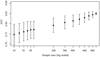 |
Fig. 2 The area under the curve (AUC) for each sample size of 1000 iterations. The black plots showed the mean AUC of each sample size, and the top and bottom arrows indicated the range of mean ± standard deviation. |
4.2 Sample size effect on habitat suitability plots
For all variables, the mean PCC positively correlated with sample size, while the standard deviation of PCC negatively correlated with sample size (Fig. 3). For depth, temperature, and velocity, the 1010 sample size models yielded the highest mean PCC (depth: 0.71; temperature: 0.83; velocity: 0.74), and the 50 sample size models showed the lowest PCC (depth: 0.18; temperature: 0.19; velocity: 0.46) (black dots in Fig. 3). For slope, the 700 sample size models yielded the highest mean PCC (0.91), and the 60 sample size models showed the lowest values (0.81). However, the standard deviation of the sample size of 700 of the slope (i.e., 0.1) is larger than that of the sample size of 1010 (i.e., 0.01). These results indicate the 1010 sample based plots of slope provided more stabilized habitat suitability plots than the 700 sample size models. Moreover, the mean PCC remained at the high level throughout all the sample size in slope; even the sample size of 50 based plots of slope yielded PCC of 0.81.
The observed ratios of the bluegill were high at depth 160 and 280 cm (the red line in Fig. 4. A-1, A-2) and the moderate slope (the red line in Fig. 4. B-1, B-2). It was high also at water temperature around 30 °C (the red line in Fig. 4. C-1, C-2). For velocity, bluegills were most abundant in the gentle flow condition, and their observed presence decreased in fast-flow sections, and then slightly increased again with a velocity around 100 cm/s (the red line in Fig. 4. D-1, D-2). The averaged habitat suitability plots of the 1010 sample size were in accordance with the observed presence; PCC calculated between the averaged habitat suitability plots of the 1010 sample size and observed presence showed a significant positive correlation with the observed presence for all variables (Tab. 1, and red and green lines in Fig. 4). Additionally, the shape of the first 100 habitat suitability plots was similar to the averaged habitat suitability plot of 1010. In case of the sample size of 50, PCC between the averaged habitat suitability plots and the observed presence showed a significant positive correlation between slope and velocity, and no significant relationship for depth and temperature (Tab. 1). Moreover, the shape of the first 100 habitat suitability plots of the sample size of 50 greatly varied among individual iterations, and they differed from the observed presence (Fig. 4).
Regarding the averaged habitat suitability plot, PCC to the observed presence showed higher values compared to the mean PCC of 1000 iterations for four variables in each sample size category (red dots in Fig. 3). For depth and temperature, the averaged habitat suitability plots of the 1010 sample size yielded the highest PCC (depth: 0.71; temperature: 0.83) among sample sizes (Tab. 1). The averaged habitat suitability plots of the sample size of 50 showed the lowest PCCs (depth: 0.61; temperature: 0.50). In contrast, slope and velocity showed different trends; for slope, the averaged habitat suitability plots of the 80 sample size models yielded the highest PCC (0.94), and that of the 1010 sample size models showed the lowest PCC (0.90) (Tab. 1). For velocity, the averaged habitat suitability plots of the sample size of 400 yielded the highest PCC (0.80), and that of the 1010 sample size models showed the lowest values (0.74). Additionally, the averaged habitat suitability plots of the 1010 sample size displayed a jagged shape, which gradually smoothed out along with the decrease of sample size (Fig. 5).
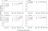 |
Fig. 3 Pearson's correlation coefficient (PCC) of four environmental variables. The black plots showed the mean PCC of 1000 iterations of each sample size, and the top and bottom arrows indicated the ranges of mean ± standard deviation. The red plots indicated PCC of the averaged habitat suitability plots, and each value was shown also in Table 1. |
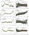 |
Fig. 4 Standardized habitat suitability plots of the 1010 and 50 sample size for four variables. The red lines indicated the observed presence. The green lines indicated the averaged habitat suitability of 1000 iterations. First 100 habitat suitability plots were shown by back line. |
The Pearson's correlation coefficient between the averaged habitat suitability and the observed ratio of the presence in all the sample size categories. Statistical significance is indicated by * p < 0.05, ** p < 0.01 and *** p < 0.001.
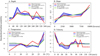 |
Fig. 5 The averaged habitat suitability plots for four variables (Standardized). The red lines indicated the observed presence. The bold blue lines indicated the averaged habitat suitability of the 1010 sample size. The green lines indicated the averaged habitat suitability of 50 sample size. Thin blue lines indicated the averaged habitat suitability of the 900-60 sample size. Statistical significance is indicated by *p < 0.05, **p < 0.01 and ***p < 0.001. |
4.3 Habitat suitability plots from pseudo-samples
The mean of averaged PCC was higher than the mean of bootstrap PCC (Tab. 2). This indicates that the averaged habitat suitability plots increase the ability to delineate habitat suitability plot, even with a small number of samples. For slope and velocity, none of the bootstrap PCC yielded negative PCC values in each pseudo-sample iteration (Tab. S3). In this case, the averaged PCC yielded higher values than the bootstrap PCC in all of the iterations (the left panel in Fig. 6).
On the other hand, for depth and temperature, negative bootstrap PCC was detected several times within 100 iterations; depth: 24 for the sample size of 50 and 19 for the sample size of 100; temperature: 19 for the sample size of 50 and 14 for the sample size of 100 (Tab. S3). In this case, the average PCC were smaller than the bootstrap PCC for the negative range while they showed the opposite pattern in the positive range (the right graph in Fig. 6).
Pearson's correlation coefficients (PCC) of Analysis (C). The bootstrap PCC; the mean of PCC calculated by 100 bootstrap iterations. The averaged PCC; PCC between the bootstrapped habitat suitability plots and the observed ratio of presence. The mean of both bootstrap PCC and averaged PCC were calculated.
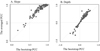 |
Fig. 6 The averaged PCCs and the bootstrap PCCs for slope and depth in case of 50 sample size. For slope, the all averaged PCCs were higher than the bootstrap PCCs. For depth, some cases showed negative PCCs, and the average PCC were smaller than the bootstrap PCC in the negative range while they showed the opposite pattern in the positive range. |
5 Discussion
5.1 Sample size effect on model performance
In the present study, the predictive performance of RF was evaluated using AUC. This value shows the predictive accuracy of “unknown” data that was not used for model construction (Liang et al., 2013). The results indicate that sample size affects the model performance; the model prediction performance is higher when we use a larger number of samples for analysis (Fig. 2). In addition, when large number of sample sizes were analyzed, the model performance stabilized, narrowing standard deviation. The previous research also revealed such dependency of model performance on sample size (Hanberry et al., 2012; Hernandez et al., 2006; Stockwell and Peterson, 2002; Wisz et al., 2008).
The AUC values calculated by the sample size 900 ranged from 0.83 to 0.87 with the mean of 0.85, indicating moderate accuracy of the RF models. This trend continued until the sample size decreased to 400. This indicates that all of the RF models generated by 900-400 samples have the potential to accurately predict the presence/absence of the bluegill. Similarly, AUC of less than 0.7 were recorded only in one iteration out of 1000 iterations when the sample size was 300, and in five iterations when the sample size was 200. However, the probability of getting AUC less than 0.7 dramatically increased when we applied less than 100 samples. Hanberry et al. (2012) investigated the change in the prediction accuracy of RF with decreasing sample size, and concluded that the performance measure begins to rapidly decrease when the sample sizes were roughly around 10–20% of the maximum sample size, which is in line with the present result.
5.2 Sample size effect on habitat suitability plots
Habitat suitability plots are also affected by sample size, similar to sample size effect on prediction performance (Fig. 3). This is reasonable because the level of uncertainty (i.e. the standard deviation of PCC of 1000 iterations) negatively correlated with sample sizes (Fig. 3). Additionally, when sample sizes are small, outliers carry more weight in analysis (Wisz et al., 2008). Thus, the ability to accurately estimate habitat suitability decreases as the sample size used for analysis decreases, which is also supported by Figure 4. These results implied that we need to be careful when generating the habitat suitability plot on the basis of a small number of samples.
Moreover, though the AUC value calculated from the sample size of 50 (Mean = 0.75, AUC of 84% trials > 0.70) indicated moderate prediction accuracy (Fig. 2), the small sample size was not adequate for drawing reliable habitat suitability plots (Fig. 4). This finding reveals that high AUC of the formulated models does not necessarily result in the generation of reliable habitat suitability plots. For these reasons, we suggest not to trust the habitat suitability plots if they are drawn from a limited number of samples. One option to overcome this limitation is to apply the averaged habitat suitability plot, which was introduced in this study.
5.3 Averaged habitat suitability plot
It is commonly difficult to increase the number of samples in the ecological survey because the number of samples is limited mainly by the cost and time (Hermoso et al., 2015b). In this research, “averaged habitat suitability plot” was developed to propose a practical method for delineating habitat suitability plots in case sample size is limited. In contrast to the great variance of habitat suitability plots among the first 100 iterations and their difference from observations with the sample size of 50 (Fig. 4), the averaged habitat suitability plots from sample sizes of 50 and 1010 (Fig. 5) were both in accordance with the reported habitat preference of bluegill. In general, bluegill is most abundant in gentle flow condition, and they prefer velocities of less than 10 cm/s (Stuber et al., 1982). Bluegill's nests are found in quiet, shallow water, and they also stay deep water sections for overwintering (Stuber et al., 1982). The optimal streambed slope for bluegill is <0.5 m/km (1/2000), and their habitat suitability decreases with an increase in slope (Stuber et al., 1982). These results demonstrated the advantage of the averaged habitat suitability plot especially for dealing with a small number of samples.
In Analysis B, PCC of the averaged habitat suitability plot (red plots in Fig. 3) was superior to the performance of the mean PCC with 1000 iterations (black plots in Fig. 3). This result might be explained by the law of large numbers. This theorem indicates that the average of the results obtained from a large number of trials should be close to the population average (Breiman, 2001). The averaged habitat suitability plots, as proposed in this study, was made by connecting the averaged estimated values for each point. Thus, the averaged habitat suitability plots more closely delineates the observed presence compared to the habitat suitability plots drawn by only one trial.
Interestingly, the averaged habitat suitability plots of the 1010 sample size showed a jagged shape, which gradually smoothed out along with the decrease of sample size (Fig. 5). This is reasonable because a large number of sample sizes contains more information compared to the small sample size. Thus, if the shape of the observed habitat suitability is complex, such as unimodal or convex, a large number of samples are required for meaningful depiction of the habitat suitability estimation. While, PCC of averaged habitat suitability plot of the 50 sample size still has high PCC (0.93, p < 0.05) in slope, and it is larger than that of the 1010 (0.90, p < 0.05). This is caused by overfitting. The result indicates that if the observed presence is a simpler shape (i.e., monotonically increase / decrease), a large number of samples might incorporate more noise into the estimated models.
In Analysis C, the mean of averaged PCC was higher compared to the mean of bootstrap PCC (Tab. 2). This indicates that the averaged habitat suitability plots increase the ability to delineate habitat suitability plots even with a small number of samples. Also, in each iteration, the averaged PCC yielded high values compared to the bootstrap PCC as long as the bootstrap PCC yielded positive values (the left panel in Fig. 6). These results indicate that the averaged habitat suitability plot improves the estimation of the habitat suitability plots.
However, further consideration needs to be done in future research. First, these averaged habitat suitability plots are highly computer intensive. Additionally, negative PCC might happen when the number of samples is limited. In this research, for depth and temperature variables, negative PCCs were recorded (Tab. S3). This might be one of the limitation of the averaged habitat suitability plot. The negative PCC is caused by insufficient information provided from a prepared sample set. The estimation yield a low degree of accuracy. However, if the samples contain important information (signals), the averaged plot might work well even with the limited number of samples.
Moreover, further consideration needs to be done for species' prevalence. Fukuda and Baets (2016) assessed the effects of data prevalence on model accuracy and habitat suitability plot using artificial species. They concluded that the data prevalence affected both model accuracy and habitat suitability plot. Specifically, habitat suitability plot obtained from a dataset with higher prevalence showed higher tolerance to unsuitable habitat conditions. Thus, further analyses for species showing different prevalence ranges, are required, and might give us more useful insight for delineating habitat suitability plots.
6 Conclusions
This study investigated the effect of sample size on habitat suitability plots using RF. The result showed that the predictive performance of the estimated RF models is positively correlated to the sample sizes. Next, we concluded that the habitat suitability plots are also affected by sample size as well as prediction performance. Especially with the sample size of 50, the estimated plots substantially varied among individual trials. To find a practical method for delineating habitat suitability plots in case that available sample data is limited, the “averaged habitat suitability plot” was proposed. The averaged habitat suitability plots based on 50 and 1010 sample sizes were in accordance with reported habitat of the bluegill. This indicates that the averaged habitat suitability plot possibly improves the estimation of habitat suitability plot even in a small number of samples. Given the difficulty to increase the number of samples in the survey, we recommend the “averaged habitat suitability plot” for better assessment of habitat suitability. Our comprehensive analysis may encourage continuous development of the application of the machine learning and visualization techniques to ecosystem management.
Supplementary Material
Supplementary Tables 1 to 3 and Figures 1 to 2. Access Supplementary Material
Acknowledgment
This research was supported by a JSPS-KAKENHI project (#15K00592, Chihiro Yoshimura).
References
- Austin MP. 2002. Spatial prediction of species distribution: an interface between ecological theory and statistical modelling. Ecol Modell 157: 101–118. [Google Scholar]
- Barbosa FG, Schneck F. 2015. Characteristics of the top-cited papers in species distribution predictive models. Ecol Modell 313: 77–83. [Google Scholar]
- Breiman L. 2001. Random forests. Mach Learn 45: 5–32. [Google Scholar]
- Cheung WWL, Lam VWY, Sarmiento JL, Kearney K, Watson R, Pauly D. 2009. Projecting global marine biodiversity impacts under climate change scenarios. Fish Fish 10: 235–251. [CrossRef] [Google Scholar]
- Conti L, Comte L, Hugueny B, Grenouillet G. 2015. Drivers of freshwater fish colonisations and extirpations under climate change. Ecography (Cop.) 38: 510–519. [Google Scholar]
- Cutler DR, Edwards TC, Beard KH, et al. 2007. Random forests for classification in ecology. Ecology 88: 2783–2792. [CrossRef] [PubMed] [Google Scholar]
- Efron B. 1979. Bootstrap methods: another look at the jackknife. Ann Stat 7: 1–26. [Google Scholar]
- Efron B, Tibshirani R. 1994. An Introduction to the Bootstrap. London: CRC Press. [CrossRef] [Google Scholar]
- Elith J, Leathwick JR, Hastie T. 2008. A working guide to boosted regression trees. J Anim Ecol 77: 802–813. [CrossRef] [PubMed] [Google Scholar]
- Fielding AH, Bell JF. 1992. A review of methods for the assessment of prediction errors in conservation presence/absence models. Environ Conserv 24: 38–49. [Google Scholar]
- Friedman J, Hastie T, Tibshirani R. 2000. Special invited paper additive logistic regression. Ann Stat 28: 337–407. [Google Scholar]
- Friedman JH. 2001. Greedy function approximation: a gradient boosting machine. Ann Stat 29: 1189–1232. [Google Scholar]
- Fukuda S. 2011. Assessing the applicability of fuzzy neural networks for habitat preference evaluation of Japanese medaka (Oryzias latipes). Ecol Inform 6: 286–295. [Google Scholar]
- Fukuda S, Baets B De. 2016. Ecological informatics data prevalence matters when assessing species' responses using data-driven species distribution models. Ecol Inform 32: 69–78. [Google Scholar]
- Greenwell BM. 2017. pdp: An R package for constructing partial dependence plots. R J 9: 421–436. [Google Scholar]
- Guisan A, Thuiller W. 2005. Predicting species distribution: offering more than simple habitat models. Ecol Lett 8: 993–1009. [Google Scholar]
- Guisan A, Tingley R, Baumgartner JB, et al. 2013a. Predicting species distributions for conservation decisions. Ecol Lett 16: 1424–1435. [Google Scholar]
- Guisan A, Tingley R, Baumgartner JB, et al. 2013b. Predicting species distributions for conservation decisions. Ecol Lett 16: 1424–1435. [Google Scholar]
- Hanberry BB, He HS, Dey DC. 2012. Sample sizes and model comparison metrics for species distribution models. Ecol Modell 227: 29–33. [Google Scholar]
- Hapfelmeier A, Ulm K. 2013. A new variable selection approach using Random Forests. Comput Stat Data Anal 60: 50–69. [Google Scholar]
- Hastie T, Tibshirani R, Friedman J. 2009. The elements of statistical learning. New York: Springer. [Google Scholar]
- Hastie TJ. 2017. Generalized Additive Models, in: Statistical Models in S. New York: Routledge, pp. 249–307 [Google Scholar]
- Hermoso V, Kennard MJ, Linke S. 2015. Assessing the risks and opportunities of presence-only data for conservation planning. J Biogeogr 42: 218–228. [Google Scholar]
- Hernandez PA, Graham C, Master LL, Albert DL. 2006. The effect of sample size and species characteristics on performance of different species distribution modeling methods. Ecography (Cop.) 29: 773–785. [Google Scholar]
- Hopkins RL, Roush JC. 2013. Effects of mountaintop mining on fish distributions in central Appalachia. Ecol Freshw Fish 22: 578–586. [Google Scholar]
- Kawanabe H, Mizuno N, Nakamura T. 2013. River Ecology. KODANSYA. [Google Scholar]
- Kim SY. 2009. Effects of sample size on robustness and prediction accuracy of a prognostic gene signature. BMC Bioinformatics 10: 4–7. [PubMed] [Google Scholar]
- Kuhn M, Wing J, Weston S, et al. 2016. Package “caret” Classification and Regression Training Description Misc functions for training and plotting classification and regression models. [Google Scholar]
- Liang L, Fei S, Ripy JB, Blandford BL, Grossardt T. 2013. Stream habitat modelling for conserving a threatened headwater fish in the Upper Cumberland River, Kentucky. River Res Appl 29: 1207–1214. [Google Scholar]
- Liaw A, Wiener M, 2015. Package ‘randomForest’. [Google Scholar]
- Mi C, Huettmann F, Guo Y, Han X, Wen L. 2017a. Why choose Random Forest to predict rare species distribution with few samples in large undersampled areas? Three Asian crane species models provide supporting evidence. PeerJ 5: e2849. [CrossRef] [PubMed] [Google Scholar]
- Mi C, Huettmann F, Sun R, Guo Y. 2017b. Combining occurrence and abundance distribution models for the conservation of the Great Bustard. PeerJ 5: e4160. [CrossRef] [PubMed] [Google Scholar]
- Michaelis J, Diekmann MR. 2017. Biased niches − species response curves and niche attributes from Huisman-Olff-Fresco models change with differing species prevalence and frequency. PLoS ONE 12: 1–16. [CrossRef] [Google Scholar]
- MLIT. 2011. River Enviromental Database [WWW Document]. [Google Scholar]
- MLIT. 2006a. Fundamental servey manual for fish. [Google Scholar]
- MLIT. 2006b. Fundamental servey manual. [Google Scholar]
- Moudrý V, Šímová P. 2012. Influence of positional accuracy, sample size and scale on modelling species distributions: a review. Int J Geogr Inf Sci 26: 2083–2095. [Google Scholar]
- Moyle PB, Light T, 1996. Biological invasions of fresh water: empirial rules and assembly theory. Biol Conserv 78: 149–161. [Google Scholar]
- Muñoz-mas R, Fukuda S, Vezza P, Martínez-capel F. 2016. Ecological informatics comparing four methods for decision-tree induction: a case study on the invasive Iberian gudgeon (Gobio lozanoi; Doadrio and Madeira, 2004). Ecol Inform 34: 22–34. [Google Scholar]
- Nakao H, Fujita K, Kawabata T, Nakai K, Sawada H. 2005. Breeding ecology of bluegill, Lepomis macrochirus, an invasive alien species, in the north basin of Lake Biwa, central Japan. Jpn J Ichthyol 53: 55–62. [Google Scholar]
- Nelder JA, Wedderburn RWM. 1972. Generalized linear models. J R Stat Soc Ser A 135: 370–384. [Google Scholar]
- Olden JD, Joy MK, Death RG. 2004. An accurate comparison of methods for quantifying variable importance in artificial neural networks using simulated data. Ecol Modell 178: 389–397. [Google Scholar]
- Onishi F. 2013. GIS Map Book for Japanese River Basin. Osaka Municipal University Press. [Google Scholar]
- R Development Core Team. 2014. R: A language and environment for statistical computing. Vienna, Austria. [Google Scholar]
- Rydgren K, Økland RH, Økland T. 2003. Species response curves along environmental gradients. A case study from SE Norwegian swamp forests. J Veg Sci 14: 869–880. [Google Scholar]
- Ryo M, Yoshimura C, Iwasaki Y. 2018. Importance of antecedent environmental conditions in modeling species distributions. Ecography (Cop.) 41: 825–836. [Google Scholar]
- Shiroyama R, Yoshimura C. 2016. Assessing bluegill (Lepomis macrochirus) habitat suitability using partial dependence function combined with classification approaches. Ecol Inform 35: 9–18. [Google Scholar]
- Stockwell DR, Peterson AT. 2002. Effects of sample size on accuracy of species distribution models. Ecol Modell 148: 1–13. [Google Scholar]
- Stuber R, Gebhart G, Maughan E. 1982. Habitat suitability index models: BLUEGILL. U.S.D.I. Fish Wildl. Serv. FWS/OBS-82. [Google Scholar]
- Swets JA. 1988. Measuring the accuracy of diagnostic systems. Science 240: 1285–1293. [Google Scholar]
- Taniguchi Y. 2012. Bluegill's effect for ecosystem. Nippon Suisan Gakkaishi 78: 991–996. [CrossRef] [Google Scholar]
- Vezza P, Muñoz-Mas R, Martinez-Capel F, Mouton A. 2015. Random forests to evaluate biotic interactions in fish distribution models. Environ Model Softw 67: 173–183. [Google Scholar]
- Wisz MS, Hijmans RJ, Li J, Peterson AT, Graham CH, Guisan A, Elith J, Dudík M, Ferrier S, Huettmann F, Leathwick JR, Lehmann A, Lohmann L, Loiselle BA, Manion G, Moritz C, Nakamura M, Nakazawa Y, Overton JMC, Phillips SJ, Richardson KS, Scachetti-Pereira R, Schapire RE, Soberón J, Williams SE, Zimmermann NE. 2008. Effects of sample size on the performance of species distribution models. Divers Distrib 14: 763–773. [Google Scholar]
- Zurell D, Elith J, Schro B. 2012. Predicting to new environments: tools for visualizing model behaviour and impacts on mapped distributions. Divers Distrib 18: 628–634. [Google Scholar]
Cite this article as: Shiroyama R, Wang M, Yoshimura C. 2020. Effect of sample size on habitat suitability estimation using random forests: a case of bluegill, Lepomis macrochirus. Ann. Limnol. - Int. J. Lim. 56: 13
All Tables
The Pearson's correlation coefficient between the averaged habitat suitability and the observed ratio of the presence in all the sample size categories. Statistical significance is indicated by * p < 0.05, ** p < 0.01 and *** p < 0.001.
Pearson's correlation coefficients (PCC) of Analysis (C). The bootstrap PCC; the mean of PCC calculated by 100 bootstrap iterations. The averaged PCC; PCC between the bootstrapped habitat suitability plots and the observed ratio of presence. The mean of both bootstrap PCC and averaged PCC were calculated.
All Figures
|
Fig. 1 Flowchart describing the analyses of this study. PCC indicate Pearson's correlation coefficient. |
| In the text | |
|
Fig. 2 The area under the curve (AUC) for each sample size of 1000 iterations. The black plots showed the mean AUC of each sample size, and the top and bottom arrows indicated the range of mean ± standard deviation. |
| In the text | |
|
Fig. 3 Pearson's correlation coefficient (PCC) of four environmental variables. The black plots showed the mean PCC of 1000 iterations of each sample size, and the top and bottom arrows indicated the ranges of mean ± standard deviation. The red plots indicated PCC of the averaged habitat suitability plots, and each value was shown also in Table 1. |
| In the text | |
|
Fig. 4 Standardized habitat suitability plots of the 1010 and 50 sample size for four variables. The red lines indicated the observed presence. The green lines indicated the averaged habitat suitability of 1000 iterations. First 100 habitat suitability plots were shown by back line. |
| In the text | |
|
Fig. 5 The averaged habitat suitability plots for four variables (Standardized). The red lines indicated the observed presence. The bold blue lines indicated the averaged habitat suitability of the 1010 sample size. The green lines indicated the averaged habitat suitability of 50 sample size. Thin blue lines indicated the averaged habitat suitability of the 900-60 sample size. Statistical significance is indicated by *p < 0.05, **p < 0.01 and ***p < 0.001. |
| In the text | |
|
Fig. 6 The averaged PCCs and the bootstrap PCCs for slope and depth in case of 50 sample size. For slope, the all averaged PCCs were higher than the bootstrap PCCs. For depth, some cases showed negative PCCs, and the average PCC were smaller than the bootstrap PCC in the negative range while they showed the opposite pattern in the positive range. |
| In the text | |
Current usage metrics show cumulative count of Article Views (full-text article views including HTML views, PDF and ePub downloads, according to the available data) and Abstracts Views on Vision4Press platform.
Data correspond to usage on the plateform after 2015. The current usage metrics is available 48-96 hours after online publication and is updated daily on week days.
Initial download of the metrics may take a while.