| Issue |
Ann. Limnol. - Int. J. Lim.
Volume 56, 2020
|
|
|---|---|---|
| Article Number | 6 | |
| Number of page(s) | 13 | |
| DOI | https://doi.org/10.1051/limn/2020004 | |
| Published online | 17 April 2020 | |
Research Article
Monitoring spatiotemporal variability of water quality parameters Using Landsat imagery in Choghakhor International Wetland during the last 32 years
1
Faculty of Fisheries and Environmental Sciences, Gorgan University of Agricultural Sciences and Natural Resources, Gorgan, Iran
2
Department of Natural Resources, Isfahan University of Technology, Isfahan, Iran
* Corresponding author: This email address is being protected from spambots. You need JavaScript enabled to view it.
Received:
15
January
2020
Accepted:
5
March
2020
Abstract
Use of Landsat is of importance in monitoring and assessment of long-term changes of water quality in freshwater ecosystems, especially in small water bodies. In this study, over a 32-year period (1985–2017), the changes in water surface temperature (WST), secchi disk transparency (SDT), and chlorophyll-a (Chl-a) concentration were estimated at the Choghakhor wetland using Landsat imagery. Based on WST three detectable temperature zones can be observed within the wetland aquatic environment where the highest amount was observed in thermal strips. The results showed Chl-a concentration volatility in different periods in the wetland as well as its long-term increasing trend. The western part of the wetland, as compared to other areas, was affected by these changes, which could be due to the human activity concentrated in this area. In contrast (SDT) showed a decreasing trend during this period that was consistent with the observed changes in Chl-a concentration. This could be due to an increase in organic matter load and suspended solids in the water body of wetland during this time. Comparison of the extracted satellite data with the field data showed the least RMSE and high R2. Also, ANOVA results showed significant spatio-temporal differences between the studied parameters in Choghakhor wetland (p < 0.05). The present study can help to detect long-term changes in Choghakhor wetland and help toward moving to optimal management and protection of this wetland.
Key words: Choghakhor International Wetland / chlorophyll-a / landsat imagery / spatio-temporal variations / water quality
© EDP Sciences, 2020
1 Introduction
Wetlands play a key role in food production, water and air purification, carbon storage and even changing local climate, affecting food turnover rate, prevention of flooding and overall protection of the biodiversity in local freshwater ecosystems (Chen et al., 2011; Ryan et al., 2012; Keddy, 2010). Conventional measurements and monitoring of water quality involve in situ sampling, which is a costly and time consuming (Ogilvie et al., 2018; El Masri et al., 2008). In addition, for tracking methods in the field, some areas are often inaccessible or difficult to sample (Chen and Quan, 2012). Due to the prevalent logistic limitations, it is not possible to cover the entire area of water or frequent sampling at a site (Chen and Quan, 2012). Overall in situ sampling encountered with some problems which inhibit coherent monitoring and estimation of water quality (Senay et al., 2001; El Masri and Rahman, 2008). In contrast, remote sensing techniques can overcome these constraints by providing alternative methods for monitoring water quality across a wide range of time and spatial scales (Senay et al., 2001; El Masri and Rahman, 2008). Remote sensing images can pass even across inland water and hence, confirming in situ measured parameters (Chen and Quan, 2012). Remote sensing analyzes the radiation data by a sensor in a specific area (here the wetland of water body). Achieved information, such as water transparency and chlorophyll-a (Chl-a) is in fact radiance within the visible and is near-infrared (Dörnhöfer and Oppelt, 2016). For example, Chl-a concentration can be measured at spectral bands of 440–560 nm and 670 nm (Matthews, 2011). In water column, the optical properties of water body such as suspended particulate matter (SPM) and Chl-a, may alter the radiation by absorption and scatter (Odermatt et al., 2012). For measuring water surface temperature (WST), sensors are needed that measure radiation at thermal infrared (13–17 μm) (Dörnhöfer and Oppelt, 2016). High resolution satellites such as Landsat are the available and efficient options for satellite-based measurements to monitor water quality even in small waters bodies (Ogilvie et al., 2018; Brezonik et al., 2005). The Landsat data series are ideal for this purpose based on a 30-meter spatial resolution, especially for some of the relatively small waters bodies (Lee et al., 2016; Brezonik et al., 2005). Landsat is freely available and contains a collection of archived data that can provide us with insights into historical events or developments in a region and therefore, can be used for monitoring purposes (Chen and Quan, 2012). Of course, estimation of qualitative parameters with Landsat has various limitations. The most prominent limitation for investigated properties within water is possessing inherent optical properties (IOPs) which can be measured through satellite sensors (Brezonik et al., 2005). Landsat measures the radiance with the sensor and cannot be calibrated with the intensity of the solar radiation, which usually varies with factors such as latitude, day length, and season. Here the atmospheric interference, which can influence reflected radiation level, is important (Brezonik et al., 2005).
In this study, we investigated the remote sensing of WST, Chl-a concentration and secchi disk transparency (SDT) parameters. WST is one of the most important abiotic factors in determining environmental changes and ecological activities of the water body (Kang et al., 2014). The physical, biological and chemical processes depend on temperature. For instance, the temperature affects the dissolve oxygen content of water, the metabolic rate of aquatic organisms (Wetzel, 2001). Chl-a is a well-known indicator of ecological health in an aquatic environment that is widely used to represent water quality and trophic status (Sun et al., 2014). Since phytoplankton contains chlorophyll, its biomass is detectable by optical sensors; hence, Chl-a is an ecological indicator for the study of the impact of nutrients and the ecosystem's status in the water body (Shutler et al., 2007). SDT is one of the parameters that can show the level of opacity in the water. It can also be used in the evaluation of the eutrophication characteristics of water body with other parameters (Yüzügüllü and Aksoy, 2011). For inland water ecosystems, SDT has been widely measured by remote sensing (e.g., Olmanson et al., 2008; Greb et al., 2009).
Permanent protection and monitoring of wetland changes, which are among the national natural assets of each country, are among the needs of sustainable development, and identifying long-term wetland changes needs to be temporally analyzed using holistic approaches such as remote sensing. That's why the present study aims to investigate and monitor temporal and spatial variations of water quality parameters such as WST, Chl-a and SDT at Choghakhor International wetland using Landsat images in 1985–2017and the results have been evaluated.
2 Materials and method
2.1 Study area
The Choghakhor international wetland, as one of the most important structural elements in the landscape of the region and important bird area (IBA), is located in Chaharmahal and Bakhtiari province, Borujen city and Boldaji district in the central Zagros Mountains, the basin of the Karun River. This wetland is located between 50° 52′ to 50° 56′E and 31° 54′ to 31° 56′N (Fig. 1). The Choghakhor wetland as one of 23 Ramsar sites in Iran with an area of 1600 ha is one of the most important sites of Iran in terms of presence of endemic endangered fish species (Aphanius vladykovi) and the type of wetland class is Lacustrine based on the Ramsar Convention (Behrouzirad, 2007; RSIS, 2010; Ebrahimi and Moshari, 2006).
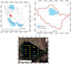 |
Fig. 1 Map and points of dataset in Choghakhor Wetland, Iran. The triangles represent dam. |
2.2 Satellite data acquisition and process
Landsat contains a large number of satellite images archive of the studied area (path /row: 164/38) from 1985 to 2017. In this study, Landsat 5, 7 and 8 satellite images (TM, ETM + and OLI sensors) were used. These images were selected based on available data from Landsat satellite archives. All images have been tried on a specific date (similar environmental conditions) to obtain better results. Most of the images are from May and October (spring and autumn, respectively). Eventually, only 18 Landsat scenes (Tab. 1) were selected. The acquired images were Level-1 and obtained from earthexplorer.usgs.gov.
In this study, geometric and radiometric correction was performed on the required images. After studying of different methods, atmospheric correction was used by DOS (Dark Object Subtraction) method. Also, based on several studies (Hicks et al., 2013; Patra et al., 2016; Bonansea et al., 2015; Urbanskia et al., 2016), this method was found to be suitable for atmospheric correction in aquatic ecosystems. DOS searches for the darkest pixel value in any band (dark objects reflect no light). This method assumes that nonzero values for water bodies are due to atmospheric path radiance. Scattering is eliminated by subtracting this value from each pixel in the band (Patra et al., 2016; Bonansea et al., 2015).
18 Landsat scenes used in this analysis.
2.3 Field data collection
Due to the use of satellite image extraction data in this study, field data need to be validated. For this purpose, the data of WST, SDT, chlorophyll-a concentration on the wetland were collected from 2006 (Ebrahimi, 2006) and 2010 (Esmaeili, 2012). All parameters of this dataset were extracted according to the standard method (APHA-AWWA-WEF, 2000). Figure 1 shows the position of the points on the map. Also based on the GPS coordinates of these points, the parameters were extracted in other years. For better comparison and proper evaluation, the data from the images were divided into two spring and autumn seasons (dry and wet) and three geographically points west, east and center.
2.4 Water discrimination
The surface of Choghakhor wetland water area was determined through using the normalized differential water index (NDWI) and the proposed algorithm by McFeeters (1996) to identify the water body of wetland and separating unrelated pixels (Alcantara et al., 2010). Ji et al (2009) suggested that NDWI can be successfully used to define and isolate the water bodies and monitoring the water range changes. According to McFeeters (1996), the threshold value for NDWI is set to zero. The NDWI is derived using green and near infrared (NIR) bands, Eq.1: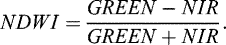 (1)
(1)
2.5 Water quality algorithm
After considering different algorithms studies, the following were selected because of suitable for small water bodies.
2.5.1 Chlorophyll-a concentration (Chl-a) and transparency (SDT) algorithms
The following relations which is suitable for small water bodies, were used to calculate Chl-a and transparency (measured as SDT) (Chao Rodríguez et al., 2014):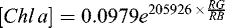 (2)
(2)
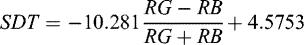 (3)where Chl-a is the chlorophyll-a concentration measured in milligrams per cubic meter (mg/m3), and SDT is the secchi disc transparency in meters.
RG and RB are the water reflectance measures in the green and blue bands, respectively.
2.5.2 Water surface temperature
Landsat thermal band was used to calculate WST. For this purpose, the digital number (DN) of thermal band must be converted to the brightness temperature. Studies in other aquatic ecosystems have also derived from this relationship (Bonansea et al., 2015; Syariza et al., 2015; Chao Rodríguez et al., 2014). Brightness temperature is calculated from sensor data using Planck's equation calibrated for thermal infrared band (according to Chander and Markham, 2003): (4)where T is temperature measured in Kelvin, Lʎ
is the thermal band spectral radiance in watts/(m2
* sr* µm), and K1 and K2 are Planck's equation coefficients which given in Table 2 for each sensor. Finally, to convert the temperature to Celsius, the number was reduced to 273.15.
(4)where T is temperature measured in Kelvin, Lʎ
is the thermal band spectral radiance in watts/(m2
* sr* µm), and K1 and K2 are Planck's equation coefficients which given in Table 2 for each sensor. Finally, to convert the temperature to Celsius, the number was reduced to 273.15.
In the case of equation (4), it should be noted that the emission coefficient for water is near to 1 and can be used to estimate water surface temperature and compare it to the dataset (Chao Rodríguez et al., 2014).
TM and ETM+ and OLI thermal band calibration constants.
2.6 Accuracy assessment
In order to validate the data obtained from the algorithms with field data (in situ), root mean square error (RMSE) and coefficient of determination (R
2) was also used (Eqs. (5) and (6)), in addition to drawing a scatter plot (Odermatt et al., 2012). (5)where, x
est are estimated water quality parameters of satellite; x
meas are measured water quality parameters of dataset; and N is the number of samples.
(5)where, x
est are estimated water quality parameters of satellite; x
meas are measured water quality parameters of dataset; and N is the number of samples. (6)where x is the estimated water quality parameters of satellite, while, y is the measured water quality parameters of dataset and n is the number of samples.
2.7 Data analyses
After extraction of parameters, normality of data was evaluated by Kolmogorov–Smirnov test (p values > 0.05 showed normality of data). The One-way ANOVA test was used to determine any significant differences among mean estimated values of water quality parameters between the years 1985 to 2017. Subsequently, the Duncan multiple range test was performed if significant differences were found in ANOVA. Differences were considered significant at p values < .05. All statistical analyses were performed using the statistical package from SPSS Inc., released 2007 (SPSS for Windows, Version 16.0, and Chicago, SPSS Inc.). All data were reported as mean ± SE (standard error).
3 Results
As mentioned in the previous section, the method used for atmospheric correction was well suited and similar to the results of other studies in aquatic ecosystems (Hicks et al., 2013; Patra et al., 2016; Bonansea et al., 2015; Urbanskia et al., 2016).
After generating the maps of each parameter, we used the scatter plots and the RMSE and R 2 metrics to validate and calibrate the data and compare it with the dataset. The results are presented in Figure 2. Accordingly, all the applied algorithms had suitable validation measurement. For WST, the RMSE of the satellite data and field data provides an error of 4.2 °C and the value of determination coefficient (R 2) with a maximum of 0.78 (y = 0.2024x + 3.57). The determination coefficient indicates a positive relationship between the variables used. Satellite measurements WST comparing to field measurements typically showed below-surface temperatures. Although there were no significant differences between satellite-based and field measurements, these differences may occur due to wind and local conditions of water. For Chl-a concentration, the amount of determination coefficient (R 2) is indicative of a high relation (0.83) among the used variables. The RMSE of the satellite data and field data provides an error of 0.47 mg/m3 (y = 0.125x + 0.521). For SDT, the amount of determination coefficient (R 2) is indicative of a high relation (0.69) among the used variables. The RMSE of the satellite data and field data provides an error of 0.38 m (y = 0.1603x + 1.5391). The results of measured parameters variation in Choghakhor wetland from 1985 to 2017 is shown from Figures 3–8. It should be noted that due to wetland drying and turbidity in the autumn of 2017, which led to dehydration, the parameter values were not reported in graph (Figs. 4, 6 and 8) at this time. Furthermore, due to the lack of available images in the autumn of 1985, the nearest month (August) was chosen as the course.
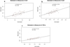 |
Fig. 2 Validation of Landsat estimated versus measured parameters (in situ) with 1:1 fit line, (a) WST, (b) SDT and (c) Chl-a. |
3.1 Water surface temperature (WST)
Figure 3 imply the spatio-temporal distribution of WST just for spring and autumn seasons of Choghakhor wetland. WST was calculated from Landsat thermal band converted to degrees Celsius. As expected, the WST map shows a spatial-temporal pattern that matches the local conditions. The warmest water of sampling time observed in high air temperature (AT) (springs) and in the north and west part of the wetland. The coldest water of sampling time found in low AT (autumns) accompanying with the center and south part of the wetland. In general, three detectable temperature zones can be observed within the wetland during studied years: less variable areas (blue in the map), moderate change areas, areas near the shoreline (red in the maps), which are called thermal strips (Sima et al., 2013). An overall view at zonation maps (Fig. 3) of the WST within study period showed WST fluctuations from 1985 to1987 (based on changes in distribution and spatial distribution on maps) were higher. Between 1995 and 2000, the wetland WST was in a relatively stable condition, which could be due to the high water volume following the construction of the dam in output of the wetland in the early 1990's and increasing rainfall during this year. During the years from 2006 to 2017, a gradual increase in the wetland of WST based on the graph was revealed (rising to a maximum of 38.5 °C in spring 2015 (Fig. 3). However, the difference of thermal band spatial resolution between different Landsat sensors in the study period (such as ETM+ versus TM resolution of thermal band) can also be considered. WST changes become more pronounced in recent years, which can affect water volume wetland as well as its margin fluctuations. This fact was observed at 38.5 °C on the margin of the wetland known as thermal string. Similar studies on other aquatic ecosystems of Iran have also found that WST range. For instance, in the study of Lake Urmia (2007–2010) by MODIS noted the maximum WST as high as 30 °C (Sima et al., 2013). The analysis of the WST graphs shows the spatial variation in different parts of the wetland (Fig. 4), in general, spring of 2015 and 2017 have a higher WST than the same time period (27.48–30.04 °C, Fig. 4). Also, WST fluctuations are higher at the west of the wetland. The lowest WST range was observed in autumns 1995, (7.7 °C, Fig. 4) which could be due to water volume in these years. ANOVA results showed a significant difference between the WST of different years in the Choghakhor wetland (p < 0.05), in Table 3. Based on maps WST (extractive data and its spatial distribution on the map) ranged from 3.3 to 38.5 °C, with a mean value of 20.9 °C.
Also, as expected, the method used to measure WST was well suited and similar to the results of other studies in aquatic ecosystems (Bonansea et al., 2015; Syariza et al., 2015; Chao Rodríguez et al., 2014).
 |
Fig. 3 Choghakhor wetland of WST (°C) changes in spring(s) and autumn (a) Season, broken down annually. |
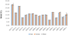 |
Fig. 4 The comparison of WST (°C) in different parts of the Choghakhor wetland in different years, spring(s) and autumn (a). |
3.2 Chlorophyll-a concentration (Chl-a)
The created images of the zoning of Chl-a concentration in Choghakhor wetland from 1985 to 2017 are shown in Figure 5, separately in spring and autumn seasons. Zoning maps of Chl-a in Choghakhor wetland, showed an increasing trend during 1985 to 2017. The highest amount of Chl-a was observed in 2006 and 2013 respectively. In general, the eastern and western parts of the wetland have more fluctuations and higher Chl-a concentration than the center (Fig. 6, which is more evident in the western regions. ANOVA results showed a significant difference between different Chl-a of different years in the Choghakhor wetland (p < 0.05), in Table 3. Based on maps Chl-a presented a mean value of 1.17 mg/m3 and relatively higher values were found in spring season. The measured Chl-a fluctuations in the Choghakhor Wetland were between 0.25 and 2.1 mg/m3. The highest Chl-a value was observed in spring season of 2006 (1.31 mg/m3).
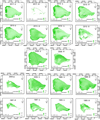 |
Fig. 5 Choghakhor wetland of Chl-a (mg/m3) changes in spring(s) and autumn (a) season, broken down annually. |
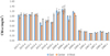 |
Fig. 6 The comparison of of Chl-a (mg/m3) in different parts of the Choghakhor wetland in different years, spring(s) and autumn (a). |
3.3 Secchi disk transparency (SDT)
The created images of zonation of SDT condition of Choghakhor wetland from 1985 to 2017 (separately in spring and autumn seasons) are presented in Figure 7. The overall depth of transparency decreased from 1985 to 2017, which indicates an increase in turbidity and suspended as well as organic particles accumulation in the wetland. It confirms the results of this study related to the Chl-a concentration increasing in recent years. Wetland of water contains high nutrient levels, suspended particulate matter and dissolved organic matter, some essential elements that cause phytoplankton growth and turbidity and decrease in SDT and increase in Chl-a were their consequences. The SDT changes in different parts of the wetland (Fig. 8) shows that the central areas of the wetland are deeper. This trend is also seen in Figure 7. It suggests higher transparency and less effect of fluctuations and wetland activities in this part of the wetland. Comparison of spring and autumn showed that the relative depth in the autumn seasons is less than those of the spring seasons. ANOVA results (Tab. 3) showed a significant difference among the SDT of different years in the Choghakhor wetland (p < 0.05). The values of SDT (based on changes in distribution and spatial distribution on maps) varied between 1.3 and 2.22 m, with a mean value of 1.71 m. This parameter also showed a seasonal variation which was related to climatic seasons and rainfall. Thus, the wetland showed the lower SDT in autumn seasons, due to the inlet of high loads of suspended solids by the inflows. While higher SDT occurred in spring seasons as inflows flows were lower. Landsat prediction, computed using equation (3) in the central pixels of the water body, provides values with a similar range.
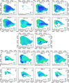 |
Fig. 7 Choghakhor wetland of SDT (m) changes in spring(s) and autumn (a) season, broken down annually. |
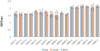 |
Fig. 8 The comparison of SDT (m) in different parts of the Choghakhor wetland in different years, spring(s) and autumn (a). |
4 Discussion
Suitable Monitoring of Choghakhor wetland changes is definitely essential for preserving this ecosystem, as a valuable natural heritage. Our study showed that remote sensing and processing of satellite images can help us to achieve this goal and this procedure could be the first study in the region that presents image of the historical changes throughout the wetlands in different periods. We also extracted several critical parameters of the aqueous environment using Landsat imagery.
Landsat is widely used to estimate water quality parameters (Dörnhöfer and Oppelt, 2016). Also, in this study, the spatio-temporal dynamics results of the qualitative parameters showed the adequate ability of Landsat. This study used three generations of Landsat (TM, ETM + and OLI) based on different years. Of course, Landsat 8 has a particular function compared to the previous Landsat sensors (Patra et al., 2016). However, Landsat's weakness is the lower temporal resolution (16-day) compared to sensors such as MODIS and Sentinel. So, in small water bodies such as Choghakor wetland, the spatial resolution (30 m) is a significant factor in monitoring of these areas. MODIS takes less temporal resolution (1 day) but with a resolution of 250 m, that it is not suitable enough for monitoring of these areas. The unique Landsat feature comparing to other sensors (such as the Sentinel with spatial resolution, 10 m and 4-year datasets since 2014) is a 40-year-old available dataset that allows long-term monitoring so it was used in the present study.
Data obtained from comparing field samplings with satellite data showed relatively good performance of RMSE (4.2 °C, 0.47 mg/m3 and 0.38 m). In a similar study at Urmia Lake, the RMSE of WST by MODIS varied between 2.59 and 0.27 °C for different years and conditions (Sima et al., 2013). The RMSE and R 2 in Arreo Lake for WST and SDT by Landsat were estimated to be 4.18 °C and 0.6 m (Chao Rodríguez et al., 2014). Also, the RMSE of WST in the two Bimont and Bariousses lakes varied between 1.75 and 2.39 °C for different conditions (Simon et al., 2014). Simon et al. (2014) found the reasons for these errors as lags in field and satellite data, differences in depth and level of temperature and satellite field data, field measurement quality, and field scale differences and thermal band resolution. In study of Kemp Lake of Texas, the R 2 of field data and Modis for chlorophyll-a were calculated 0.3 and 0.8 in spring (June) and autumn (October), respectively (El Masri and Rahman, 2008). They confirmed that the number of field samples, changes in chlorophyll-a absorption, less field data fluctuation of chlorophyll-a compared to October, as potential contributors to the weakness of R2 with field and satellite data in June.
In general, the difference in WST depends on the various conditions. The WST measured by the satellite covers an area, while field data is a point value that can lead to a meaningful difference. Also, an error in the field measurement may occur. However, WST changes are much lower than land surface temperature. Another factor is water depth. Based on the water thermal properties, wherever the depth is greater, there is a higher heat storage capacity, causing the WST to increase significantly during the warm seasons or decrease during the cold season (Fazelpoor et al., 2015), which in Choghakhor wetland, due to less fluctuations in depth and also less depth range, is not very effective. In addition, WST has a significant relationship with the characteristics of the ecosystem and is affected by environmental and climate change (Adrian et al., 2009). The highest water WST based on the graph in both seasons (spring and autumn) was observed in the western region of Choghakhor wetland (Fig. 4), which is likely to be affected by input water temperature due to agricultural activities, depth and presence of dark-colored aquatic plants. In the case of comparing several parts of the wetland, the highest WST was observed in the coastal areas of the wetland. The WST of the wetland in the spring season is higher than the autumn season, which is justified by the warmer air temperatures in the warm seasons. WST in parts with high variation can be related to wetland margins and water volume changes or the absence or presence of aquatic plant cover. According to the satellite images in the autumn seasons of 1985, 2015, and 2017, along with low water levels, the increase in WST is evident, and in winter 1995 the lowest WST is observed along with the high water status in the wetland. Interpretation the results of quantitative parameters such as Chl-a needs to understand the ecology and optical patterns in the region (Stumpf et al., 2003). In a healthy ecosystem, naturally all ecological and biological factors fluctuate due to seasonal and temporal changes, and the intensity of this fluctuation varies with respect to the geographical location, extent, depth, dominant flows and shape of the water source. The Choghakhor wetland is no exception. Considering to the variations of Chl-a among different seasons in the studied years, Chl-a concentration is higher in spring than the autumn, which is similar to the fluctuations of aquatic ecosystems in temperate regions and follows the natural pattern of primary production in these areas. In the study by Esmaeili (2012) in the Choghakhor Wetland, Chl-a patterns were similar to those in this study, and this parameter was higher in spring. Although it increased slightly in the autumn, but still was lower than the spring (Esmaeili, 2012). In general, Chl-a concentration is dependent on biomass of phytoplankton and its mean concentration in aquatic ecosystems is a function of mean total phosphorus and presents a log-log relationship. According to the several studies, there is a positive correlation between Chl-a concentration and nutrients (Wetzel, 2001; Souchu et al., 2010; Pereira et al., 2010; Iqbal et al., 2017; Primpas et al., 2010). These changes vary in parameters such as Chl-a and SDT in different ecosystems and may be related to the lack of nitrogen at high phosphorus levels, the impact of organic solid particles, and their rate of washing. (Kufel et al., 1997; Carpenter, 2005; Covino et al., 2009; Zoriasatein et al., 2013). Regarding the years when Chl-a concentration was higher in autumn than in spring (1985, 1987, and 2013), environmental conditions in the area should be studied and environmental factors, especially water turbulence and water temperature, are usually influenced by water volume fluctuations, especially in the years 1985–1987 (years before dam construction). However, further study of aquatic ecosystems shows that the relationship of Chl-a with phosphorus and transparency in sediment reservoirs is more unstable than similar lakes and ecosystems (Boynton et al., 1982; Filstrup and Downing, 2017; Murrell et al., 2007). Stumpf et al. (2003) found that Chl-a concentration and algae density in the east of the Gulf of Mexico increased from late summer to early winter. SDT changes can be observed in relation to Chl-a fluctuations and these changes must be evaluated from two aspects: (i) Inflows into the wetland (organic and inorganic suspensions and associated particles), as observed in the wetland center at most of the years it was more transparent, (ii) Density of phytoplankton (based on Chl-a concentration) that increases or decreases as a result of transparency changes. However, the results of this study showed that SDT was more influenced by the second factor (phytoplankton density). Residential and agricultural uses of the Choghakhor wetland are dispersed in the southern part of the wetland, where the waste water is transferred from the sources into the wetland. In the northern half of the wetland, the use of pollutants or wastewater and the source of input that is derived from it, is very low and almost contained bare land (Samadi, 2015). Therefore, the amount of nutrients in this area of Choghakhor wetland can be attributed to the reasons for the increase of Chl-a concentration. Also, in autumn, with the lowest degree of transparency, the highest density of phytoplankton and Chl-a was observed. It seems that the existing parameters are insufficient to investigate the dominant relationships within wetland ecosystem, and some factors make the analysis difficult to complete, such as: (1) highly dependent variables of the studied variables (nutrients, chlorophyll and phytoplankton, transparency (SDT)), (2) Seasonal changes of nutrients in phytoplankton densities, 3) difficulty in separating extrinsic factors (phytoplankton and nutrients are instinct factors of aquatic ecosystems structures), 4) Nutrition cycle dynamic and identifying factors resulting from human activities should be added.
5 Conclusions
Our method helps to have a rapid detection of ecological changes in the wetland by using some environmental indicators (through extraction of satellite images). The results showed Chl-a and SDT volatility in different periods. Chl-a. during 1985 to 2017 showed an increasing trend that was consistent with changes in SDT. The western part of the wetland, as compared to other areas, was affected by these changes, which could be due to the human activity concentrated in this area. Although it was not possible to draw profiles from the temperature of wetland depth with the method used in this study, it provides valuable information based on the epilimnion layer, as well as patterns and spatial-temporal distribution of WST in different years (1985–2017). Furthermore, combining in situ data and satellite data can fill the gaps of our information in this ecosystem and help us toward comprehensive management of these valuable resources and represent an outlook from the past to the present. The information obtained from the present study could be helpful in the future optimal management of wetlands (exposed to climate change, pollution, etc.). Mapping the spatial distribution for Chl-a, SDT, and WST with remotely sensed data would be helpful for management of water bodies by determining the point and non-point sources of pollutions that are responsible for such spatial variability. Thus, we conclude that remote sensing can potentially be used as a tool for monitoring water quality throughout the seasons and can provide natural resource managers and decision makers with crucial information. Future research should focus more on the use of remotely sensed data to estimate viability seasonal variations in water quality parameters in long-term and their potential impact as an approach to mitigate climate change.
Funding
This study was funded by the Iran National Science Foundation (INSF) [grant number 97008261]. Also, this research was financially supported by Gorgan University of Agricultural Sciences and Natural Resources (GAU), Gorgan, Iran.
Acknowledgments
We thank Iran National Science Foundation (INSF) and Gorgan University of Agricultural Sciences and Natural Resources (GAU), Gorgan, Iran for their support.
References
- Adrian R, O'Reilly CM, Zagarese H, et al. 2009. Lakes as sentinels of climate change. Limnol Oceanogr 54: 2283–2297. [CrossRef] [PubMed] [Google Scholar]
- APHA–AWWA–WEF (American Public Health Association–American Water Works Association–Water Environment Federation). 2000. Standard methods for the examination of water and wastewater (18th ed.). APHA–AWWA–WEF: Washington, DC. [Google Scholar]
- Alcantara EH, Stech JL, Lorenzzetti JA, et al. 2010. Remote sensing of water surface temperature and heat flux over a tropical hydroelectric reservoir. Remote Sens Environ 114: 2651–2665. [Google Scholar]
- Bonansea M, Rodriguez MC, Pinotti L, Ferrero S. 2015. Using multi-temporal Landsat imagery and linear mixed models for assessing water quality parameters in Río Tercero reservoir (Argentina). Remote Sens Environ 158: 28–41. [Google Scholar]
- Brezonik P, Kevin D, Bauer M, Bauer M. 2005. Landsat-based remote sensing of lake water quality characteristics, including chlorophyll and colored dissolved organic matter (CDOM). Lake Reserv Manag 21: 373–382. [CrossRef] [Google Scholar]
- Behrouzirad B. 2007. Wetlands of Iran, Tehran, Iran. [Google Scholar]
- Boynton WR, Kemp WM, Keefe CW. 1982. A comparative analysis of nutrients and other factors influencing estuarine phytoplankton production. In: V.S. Kennedy (ed.), Estuarine Comparisons. New York: Academic Press, p. 69–90. DOI: 10.1016/B978-0-12-404070-0.50011-9. [CrossRef] [Google Scholar]
- Carpenter SR. 2005. Eutrophication of aquatic ecosystems: Bistability and soil phosphorus. Proc. Natl Acad Sci 102: 10002–10005. [CrossRef] [Google Scholar]
- Covino T, Golden HE, Li HY, Tang J. 2009. Aquatic carbon-nutrient dynamics as emergent properties of hydrological, biogeochemical, and ecological interactions: scientific advances. Water Resour Res 54:7138–7142. [Google Scholar]
- Chander G, Markham BL. 2003. Revised Landsat-5 TM radiometric calibration procedures and postcalibration dynamic ranges. IEEE Trans. Geosci. Remote Sens. 41: 2674–2677. [Google Scholar]
- Chao Rodríguez Y, Anjoumi A, Domínguez Gómez JA, Rodríguez Pérez D, Rico E. 2014. Using Landsat image time series to study a small water body in Northern Spain. Environ Monitor Assess 186: 3511–3522. [Google Scholar]
- Chen J, Quan W. 2012. Using Landsat/TM imagery to estimate nitrogen and phosphorus concentration in Taihu Lake, China. IEEE J Stars 5: 273–280. [Google Scholar]
- Chen ZH, Mao ZH, Chen JY. 2011. Coastline change monitoring using 4 periods' remote Sensing data in Zhejiang Province from 1986 to 2009. Appl Remote Sens Technol 26: 68–73. [Google Scholar]
- Dörnhöfer K, Oppelt N. 2016. Remote sensing for lake research and monitoring − recent advances. Ecol Indic 64: 105–122. [Google Scholar]
- Ebrahimi E. 2006. Using GIS Techniques in Aquatic Environment Studies: Developing Databases and Map for Choghakhor Wetland. University project research, No, 2887, Department of Natural Resources, Isfahan University of Technology, 80 p. [Google Scholar]
- Ebrahimi S, Moshari M. 2006. Evaluation of the Choghakhor Wetland status with the emphasis on environmental management problems. Publications of the Institute of Geophysics. Polish Acad Sci E-6 (390) 8pp. [Google Scholar]
- Esmaeili AR. 2012. Trophic Status of Choghakhor Wetland, Thesis of Master of Science, Department of Natural Resources, Isfahan University of Technology, 87 p. [Google Scholar]
- El Masri B, Rahman AF. 2008. Estimation of water quality parameters for Lake Kemp Texas derived from remotely sensed data. Available online at twri.tamu.edu/funding/usgs/2006-07/el-masri_manuscript.pdf [Google Scholar]
- Fazelpoor K, Dadolahi Sohrab A, Elmizadeh H, Asgari HM, Khazaei SH. 2015. Evaluating the Efficiency of the Use of Satellite Images in Measuring the Sea Surface Temperature and Carbon Fixation in the Persian Gulf. Tech J Eng Appl Sci 5: 242–254. [Google Scholar]
- Filstrup CT, Downing JA. 2017. Relationship of chlorophyll to phosphorus and nitrogen in nutrient-rich lakes. Inland Waters 7: 385–400. [Google Scholar]
- Greb SR, Martin AA, Chipman JW. 2009. Water clarity monitoring of lakes in Wisconsin, USA using Landsat, in Proceedings of 33rd International Symposium of Remote Sensing of the Environment. Stresa, Italy. [Google Scholar]
- Hicks BJ, Stichbury GA, Brabyn LK, Allan MG, Ashraf S. 2013. Hindcasting water clarity from Landsat satellite images of unmonitored shallow lakes in the Waikato region, New Zealand. Environ Monitor Assess 185: 7245–7261. [CrossRef] [Google Scholar]
- Iqbal M, Billah M, Haider N, Islam Sh, Payel HR. 2017. Seasonal distribution of phytoplankton community in a subtropical estuary of the south-eastern coast of Bangladesh. Zool Ecol 27(3-4), https://doi.org/10.1080/21658005.2017.1387728. [Google Scholar]
- Ji L, Zhang L, Wylie B. 2009. Analysis of dynamic thresholds for the normalized difference water index. Photogram Eng Remote Sens 75: 1307–1317. [CrossRef] [Google Scholar]
- Kang K, Kim SH, Kim D, Cho YK, Lee SH. 2014. Comparison of coastal sea surface temperature derived from ship, air, and space-borne thermal infrared systems. Int Geosci Remote Sens Symp: 4419–4422. [Google Scholar]
- Keddy PA. 2010. Wetland Ecology: Principles and conservation. Cambridge University Press. [CrossRef] [Google Scholar]
- Kufel L, Prejs A, Rybak JI (Eds.). 1997. Shallow Lakes '95: Trophic Cascades in Shallow Freshwater and Brackish Lakes (Developments in Hydrobiology) Dordrecht: Springer, Vol. 119 [CrossRef] [Google Scholar]
- Lee Z, Shang S, Qi L, Yan J, Lin G. 2016. A semi-analytical scheme to estimate Secchi-disk depth from Landsat-8 measurements. Rem Sens Environ 177: 101–106. [CrossRef] [Google Scholar]
- Matthews MW. 2011. A current review of empirical procedures of remote sensing in inland and near-coastal transitional waters. Int J Remote Sens 32: 6855–6899. [Google Scholar]
- McFeeters SK. 1996. The use of the Normalized Difference Water Index (NDWI) in the delineation of open water features. Int J Remote Sens 17: 1425–1432. [Google Scholar]
- Murrell MC, Hagy JD, Lores EM, Greene RM. 2007. Phytoplankton production and nutrient distributions in a subtropical estuary: importance of freshwater flow. Estuar Coasts 30: 390–402. [CrossRef] [Google Scholar]
- Odermatt D, Gitelson A, Brando VE, Schaepman M. 2012. Review of constituentretrieval in optically deep and complex waters from satellite imagery. Rem Sens Environ 118: 116–126. [CrossRef] [Google Scholar]
- Olmanson LG, Bauer ME, Brezonik PL. 2008. A 20-year Landsat water clarity census of Minnesota's 10, 000 lakes. Remote Sens Environ 112: 4086–4097. [Google Scholar]
- Ogilvie A, Belaud G, Massuel S, Mulligan M, Le Goulven P, Calvez R. 2018. Surface water monitoring in small water bodies: potential and limits of multi-sensor Landsat time series. Hydrol Earth Syst Sciences 22: 4349–4380. [CrossRef] [Google Scholar]
- Patra P, Dubey SK, Kumar Trivedi R, Kumar Sahu S, Keshari Rout S. 2016. Estimation of Chlorophyll a concentration and trophic states for an inland lake from Landsat 8 OLI data: a case of Nalban Lake of East Kolkata Wetland, India. doi: 10.20944/preprints201608.0149.v1. [Google Scholar]
- Pereira HC, Allott N, Coxon C. 2010. Are seasonal lakes as productive as permanent lakes? A case study from Ireland. Can J Fish Aquatic Sci 2010: 1291–1302. [CrossRef] [Google Scholar]
- Primpas I, Tsirtsis G, Karydis M, Kokkoris GD. 2010. Principal component analysis: development of a multivariate index for assessing eutrophication according to the european water framework directive. Ecol Indic 10: 178–183. [Google Scholar]
- Ramsar Sites Information Service (RSIS). 2010. Choghakhor Wetland. https://rsis.ramsar.org/ris/1939?language=en. [Google Scholar]
- Ryan PP, Geoffrey JH, Gang C. 2012. How wetland type and area differ through scale: a geobia case study in Alberta's Boreal Plains. Remote Sens Environ 117: 135–145. [Google Scholar]
- Samadi J. 2015. Survey of spatial-temporal impact of quantitative and qualitative of land use wastewaters on Choghakhor wetland pollution using IRWQI index and statistical methods. Iran Water Resour Res 11: 157–191. [Google Scholar]
- Senay GB, Shafique NA, Autrey BC, Fulk F, Cormier SM. 2001. The selection of narrow wavebands for optimizing water quality monitoring on the Great Miami River, Ohio using Hyperspectral Remote Sensor Data. J Spat Hydrol 1: 1–22. [Google Scholar]
- Shutler JD, Land PE, Smyth TJ, Groom SB. 2007. Extending the MODIS 1 km ocean colour atmospheric correction to the MODIS 500 m bands and 500 m chlorophyll-a estimation towards coastal and estuarine monitoring. Rem Sens Environ 107: 521–532. [CrossRef] [Google Scholar]
- Sima S, Ahmadalipour A, Tajrishy M. 2013. Mapping surface temperature in a hyper-saline lake and investigating the effect of temperature distribution on the lake evaporation. Rem Sens Environ 136: 374–385. [CrossRef] [Google Scholar]
- Simon RN, Tormosa T, Danisb PA. 2014. Retrieving water surface temperature from archive LANDSAT thermal infrared data: application of the mono-channel atmospheric correction algorithm over two freshwater reservoirs. Int J Appl Earth Observ Geoinfor 30: 247–250. [CrossRef] [Google Scholar]
- Souchu P, Bec B, Smith VH, et al. 2010. Patterns in nutrient limitation and chlorophyll a along an anthropogenic eutrophication gradient in French Mediterranean coastal lagoons. Can J Fish Aquatic Sci 67: 743–753. [CrossRef] [Google Scholar]
- Sun D, Hu C, Qiu Z, Cannizzaro JP, Barnes BB. 2014. Influence of a red band-based water classification approach on chlorophyll algorithms for optically complex estuaries. Rem Sens Environ 155: 289–302. [CrossRef] [Google Scholar]
- Stumpf RP, Culver ME, Tester PA, et al. 2003. Monitoring Karenia brevis blooms in the Gulf of Mexico using satellite ocean color imagery and other data. Harmful Algae: 147–160. [Google Scholar]
- Syariza MA, Jaelania LM, Subehie L, Pamungkasb A, Koenhardonoc ES, Sulisetyonod A. 2015. Retrieval of Sea Surface Temperature Over Poteran Island Water of Indonesia with Landsat 8 TIRS Image: A Preliminary Algorithm, The International Archives of the Photogrammetry, Remote Sensing and Spatial Information Sciences, Volume XL-2/W4, 2015, Joint International Geoinformation Conference, 28–30 October 2015, Kuala Lumpur, Malaysia. [Google Scholar]
- Urbanskia JA, Wochnaa A, Bubakb I, et al. 2016. Application of Landsat 8 imagery to regional-scale assessment of lakewater quality, Int J Appl Earth Observ Geoinfor 51: 28–36. [CrossRef] [Google Scholar]
- Wetzel RG. 2001. Limnology: Lake and river ecosystems. San Diego, CA: Academic Press, 3rd ed. p. 1006. [Google Scholar]
- Yüzügüllü O, Aksoy A. 2011. Determination of Secchi Disc depths in Lake Eymir using remotely sensed data. Proc Social Behav Sci 19: 586–592. [CrossRef] [Google Scholar]
- Zoriasatein N, Jalili S, Poor F. 2013. Evaluation of ecological quality status with the trophic index (TRIX) values in coastal area of Arvand, northeastern of Persian Gulf, Iran. World J Fish Mar Sci 5: 257–262. [Google Scholar]
Cite this article as: Pirali Zefrehei AR, Hedayati A, Pourmanafi S, Beyraghdar Kashkooli O, Ghorbani R. 2020. Monitoring spatiotemporal variability of water quality parameters Using Landsat imagery in Choghakhor International Wetland during the last 32 years. Ann. Limnol. - Int. J. Lim. 56: 6
All Tables
All Figures
|
Fig. 1 Map and points of dataset in Choghakhor Wetland, Iran. The triangles represent dam. |
| In the text | |
|
Fig. 2 Validation of Landsat estimated versus measured parameters (in situ) with 1:1 fit line, (a) WST, (b) SDT and (c) Chl-a. |
| In the text | |
|
Fig. 3 Choghakhor wetland of WST (°C) changes in spring(s) and autumn (a) Season, broken down annually. |
| In the text | |
|
Fig. 4 The comparison of WST (°C) in different parts of the Choghakhor wetland in different years, spring(s) and autumn (a). |
| In the text | |
|
Fig. 5 Choghakhor wetland of Chl-a (mg/m3) changes in spring(s) and autumn (a) season, broken down annually. |
| In the text | |
|
Fig. 6 The comparison of of Chl-a (mg/m3) in different parts of the Choghakhor wetland in different years, spring(s) and autumn (a). |
| In the text | |
|
Fig. 7 Choghakhor wetland of SDT (m) changes in spring(s) and autumn (a) season, broken down annually. |
| In the text | |
|
Fig. 8 The comparison of SDT (m) in different parts of the Choghakhor wetland in different years, spring(s) and autumn (a). |
| In the text | |
Current usage metrics show cumulative count of Article Views (full-text article views including HTML views, PDF and ePub downloads, according to the available data) and Abstracts Views on Vision4Press platform.
Data correspond to usage on the plateform after 2015. The current usage metrics is available 48-96 hours after online publication and is updated daily on week days.
Initial download of the metrics may take a while.